Computable Performance Metrics
Module 2: Computing Error and Work Estimators
Module Author
Kris Stewart
Computer Science Department
URL stewart.sdsu.edu/
W.M. Keck Foundation
This file:
ComputablePerformanceMetrics2.htm
Overview:
Many of the calculations performed these days benefit from the methods of numerical analysis with their proven error analysis. An excellent text is Numerical Methods and Software [1] providing a careful balance between algorithms and their usefulness on modern computers, the development of the error properties of these algorithms and the impact of the implementation of the algorithm in a computer language, FORTRAN, in a portable manner so that the text, and its codes, can be applied to the wide variety of computing systems available now. The current module will augment this treatment by pursuing computationally measurable performance metrics, such as accuracy and cost that can be computed during the solution process.
Our metric for cost will be the CPU-time for the task. Our metric for accuracy will be the norm of the error, the difference between the true solution and the computed solution; therefore we limit ourselves in this exposition to problems with known solutions. The problem class to be explored is from the numerical solution of differential equations because we feel this links the mathematical theory predicted for the algorithm with an actual computable measure of performance nicely and is a problem class of interest to computational science.
We begin with the 1d solution of the boundary value problem
u’’(x) = f(x), u(0)=1, u(1)=1
with f(x) = -(2 π)2
sin(2π x), so that true solution
is given by u(x) = sin (2π x). We are following an excellent lesson prepared
by Professor Matt W. Choptuik, Professor of Physics & Astronomy, ![]()
Introduction
to problem:
In this module, we demonstrate a way to compute performance statistics that are related to the mathematical predictions of the approximation formulas from numerical analysis. We examine the error due to finite difference approximation of the derivative which is expected to be O (∆x2 ) for the uniform discretization ∆x = 1/N, where N = 2level for the sequence of grids, level = 4, 5, …, 20, therefore values of N = 16, 32, …, 1048578. We also examine the work performance to solve the tridiagonal linear system of equations for this sequence of grid spacings. The known number of arithmetic operations for applying the Gaussian Elimination algorithm to the matrix with this known sparsity structure is O(N) for the adds and multiplies. We recognize that we must consider the cost for fetching the values from memory or from cache, and storing the result value back to memory. These costs will depend on the compiler and the computer architecture where the program is run. These costs are difficult to predict in advance. Therefore, we focus on the known Op Count for arithmetic and seek validation from the run-time CPU time. We hope to discover: For what value of N will the arithmetic costs come to dominate the other issues of memory access?
Statement
of the problem:
Relating performance of Gaussian Elimination for tridiagonal linear systems using known algorithm operation counts for work with the measurable run-time data of an implemented code is explored. We expect the linear work for a problem of size N to be represented as
Work (N) = c N,
for some constant c. When
we double the number of points, we expect the work to double, i.e. take twice
as long to compute.
We expect quadratic accuracy proportional to the square of our grid spacing, ∆x, or inversely proportional to the square of the problem size, given by
Accuracy (N) = d ∆x2 = d 1/N2
for some constant d. When we double the number of points, we expect
the error to decrease by a factor of 4, i.e. multiply the error by a factor of ![]()
We use the standard finite difference approximation of
u’’(xi) ~ (ui+1 – 2*ui + ui-1)/∆x2,
xi = i*∆x,
ui+1 ~ u(xi+1)
and examine a sequence of grid-sized levels,
N = 2level, level = 4, 5, … 20.
Our overall expectations of performance may be described using the ratios of the successively finer grids. For example, in the case for N=16 and N=32
Accuracy(16) ~ d (1/16)2
and
Accuracy(32) ~ d (1/32)2 ~ 2 -2 Accuracy(1/16)
Computing their ratio and taking the Log2 yields the exponent of change, one (1) for the linear measure of work and two (2) for the quadratic measure of accuracy.
Log2 ([Accuracy(coarse grid) / Accuracy(fine grid)] ) ~ 2
Log2 ([Work(coarse grid) / Work(fine grid)] ) ~ -1
Our computational task is to attempt to verify the quadratic relationship for accuracy using the known true solution to compute the error and discover the value of N where this occurs. In the same program, we expect to verify the linear work to solve a tridiagonal system of linear equations.
Solution
methodology:
We use equally spaced grid points on [0,1]
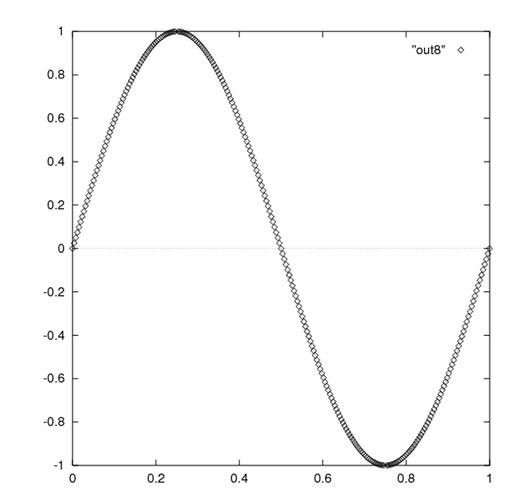
This solution was computed by Dr. Matt Choptuik and is
available from his home page http://laplace.physics.ubc.ca/People/matt/Teaching/04Fall/PHYS410/Doc/linsys/ex2/soln8.ps. Dr. Choptuik’s
class lesson was the starting point for the code used to demonstrate this
module’s computable metrics of
accuracy and work. We used GhostScript
[5] to view the postscript files from Dr. Choptuik’s class page and SnagIt [6]
to capture the image as PGN (portable network graphic) above to include in this document.
Dr. Choptuik’s class page also
presents the plot of the error for varying grids of level = 5, 6 and 7 reproduced in this module.
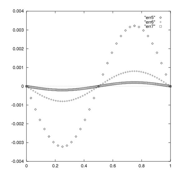
http://laplace.physics.ubc.ca/People/matt/Teaching/04Fall/PHYS410/Doc/linsys/ex2/err567.ps
Assessment
of how well the model solves the problem:
We are indebted to Professor Matthew Choptuik, Dept of
Physics and Astronomy,
Empirical
data:
Table 1 presents the results from running kbvp1d-single.f with the single precision LAPACK subroutine SGTSV. Also on Table 1 are the known eigenvalues for the matrix A, found online through a Google search described in the references [7]. Notice the shaded rows of the table (in the Word document) when level ≥ 8. These are untrustworthy due to the ill-conditioning of the matrix A and the natural propagation of round-off error in the computation. Round-off error was covered in Modules 0 and 1 of this set of notes.
Conceptual
questions to examine student’s understanding:
Did you notice a
consistency in the behavior of the work performance metric in Table 1?
Student should notice that the Work Ratio column shows a smooth value of ½ = 2-1, which would be expected for a linear algorithm doing Gaussian Elimination on a tridiagonal system of equations. The computed exponent is a smooth value of -1.0 validating that Work is inversely proposal to problem size.
Note: student should begin to feel comfortable examining these computed values and understanding that log2(1/2) = -1, which is our expect work performance metric for a linear algorithm.
Did you notice a
consistency in the behavior of the accuracy performance metric, the Error
Ratio, in Table 1?
Students should notice that the first 4 rows, do provide a smooth
result. The number of grid points is
doubled, N → N*2 or ∆x
→ ![]() , and we expect the accuracy to be make smaller by a factor
of
, and we expect the accuracy to be make smaller by a factor
of ![]() or a factor of 4 for
the quadratic grid approximation used for the finite difference. Taking the ratio of the coarse-grid approximate
to the fine-grid approximate, we compute the Error Ratio of roughly 4 with the
exponent of 2, for the first four rows of Table 1 (level = 4, 5, 6, 7).
or a factor of 4 for
the quadratic grid approximation used for the finite difference. Taking the ratio of the coarse-grid approximate
to the fine-grid approximate, we compute the Error Ratio of roughly 4 with the
exponent of 2, for the first four rows of Table 1 (level = 4, 5, 6, 7).
After the fourth row of Table 1, we have a grid-spacing of h = ∆x = 0.0078125. We are reaching a limitation that comes from the ill-conditioning of the linear system of equations. For the current problem with N = 4, our matrix is
A = 
The matrix A has a large magnitude eigenvalue
λ1 = -2 { 1 + cos (π/N) } ~ -4
and small magnitude eigenvalue
λN =
-2 { 1 + cos ({N-1)π/N } ~ -h2
The explicit formula for these eigenvalues was found online [7]. The eigenvalues determine the condition number of a symmetric matrix such as this [8]. Please see the discussion under Tables 1 and 2.
Problems
and projects:
Students can be asked to use a double precision version of the same experiment. The results are presented in Table 2 running kbvp1d-double.f with the double precision LAPACK code, DGTSV. These results are shaded in rows 11 to 17 indicating their untrustworthiness, as we saw in the single precision results for smaller values of N.
Solutions:
We take the problem cited above and use the FORTRAN code kbvp1d-double.f, included in the zipfile with this module, to approximate the solution [2] for this module. This code sets up the boundary value problem above, set in a way so that the true solution is known and computed. We modified the original code to examine a sequence of grids, for levels 4 up to 12, giving N = 2level + 1, i.e. N = 17, 33, 65, 129, 257, 513, 1025, 2049, 4097, 8193, 16385, 32769, 65537, 131073, 262145, 524289, and 1048577. The sample code uses the LAPACK tridiagonal system solver, DGTSV. The code uses the UNIX utility, dtime [9]. The zipfile also contains files to compile and link with the high performance Sun subroutine library.
Suggestions
to instructors for using the module:
It is tempting to try to cover too much in a module such as this. It is a challenge to distinguish for the students how simplifications have been made without compromising the actual solution process. In the past, the author used this module to motivate students to discover the relationship between the mathematical theory that states Gaussian Elimination can be performed in O(N3) operations for a dense matrix and the observed performance in computing the numerical solution. Students are often familiar with Gaussian Elimination for dense systems and can believe the Op Count through an easy lecture, but it is a mistake to try to treat the example of the boundary value problem as dense due it has known sparsity structure. We have observed that students will continue to use computational techniques learned in class for problem solving later in their career. They do not remember your caveat “This is only for a class example, you would never use dense Gaussian Elimination for this problem in practice”. We now feel that it is better to use the special case of tridiagonal systems with their linear operation count for cost.
We also recommend referring to u(x) so that later one can ease into the 2d problem as u(x,y). Our students just are not comfortable with y(x) and then later u(x,y(x)) and its dependencies, so a careful choice of notation at the start will pay off later.
Searching for a suitable problem to generate Au=b, it was easy to select the diffusion equation with its computational molecule to approximate
∂2u(xi)
/ ∂x2 ~ ![]()
at xi = x0 + i*∆x for the uniform spacing ∆x dividing the domain into N equal intervals.
An interesting source of a wide variety of computational molecules is available from of Abramowitz & Stegun, now available on-line[10]. We present formula 25.3.23 here.
It was an interesting find to see how many problems from physics are approximated by this same linear system. A nice lecture is presented in [11] for the Two-Mass Vibrating System by Professor Erik Cheever.
Consideration should be put into the prerequisites that you
might want to require for a course, or a module such as this. In the university setting, the content of
courses is always dynamic and there is a time-dependency on the correspondence
between a syllabus, a catalog description and what is actually covered in a
course. For this module, we use
We note an interesting curricular investigation for any instructor to pursue to better understand the situation at your local institution. If you require a course as a prerequisite for your own course, be clear in your own mind about precisely which topic from that prerequisite course you really expect students to understand. Then, take the time to speak with the faculty member at your school who currently teaches the course. Ask them how they cover this topic. Do they motivate the topic? With what example? Think to yourself how well this treatment prepares students for your course. You can then try to convince the other instructor teaching the prerequisite of your course to see the value of orienting their course to be aligned more smoothly with your needs. If this is not successful, you will want to spend time in your course to develop the concept more before pursuing this example.
Instructors will want to have a good relationship with the System Adminstrator of the computer used for instruction. This module will benefit from using the largest possible vector sizes to have the full range of computed metric values to make a convincing argument. At SDSU, we needed an increment in our Storage Limit for student accounts.
References:
[1] Numerical Methods and Software, D. Kahaner, C. Moler and S. Nash, Prentice-Hall, 1989. Although this text is somewhat dated, using the FORTRAN routines from LinPACK, the treatment of linear systems, the condition number of the matrix and the behavior of its error is very well written and appropriate for this module.
[2] Professor M.W. Choptuik, Physics 410: Computational Physics Course Notes, Fall 2004, Linear Systems. http://laplace.physics.ubc.ca/People/matt/Teaching/04Fall/PHYS410/Notes.html
[3] LAPACK Users’ Guide, 3rd Edition,
http://www.netlib.org/lapack/lug/
[4] DGTSV tridiagonal system solver from LAPACK. Available online from
http://www.netlib.org/lapack/double/dgtsv.f
[5] Ghostgum Software Pty Ltd, provides a shareware code to view postscript files that we have used for a while. Many other providers are possible. http://www.ghostgum.com.au/
[6] SnagIt Screen Capture software from TechSmith. http://www.techsmith.com/snagit.asp
[7] Eigenvalues of discretization matrix available from Math Forum discussion on line at
http://mathforum.org/kb/thread.jspa?threadID=1415533&messageID=4926102
This was an interesting Google search. I remembered from my first numerical analysis course, using the excellent text, Numerical Analysis: A Second Course [8] by Ortega, that the closed form formula for these eigenvalues was presented. My copy of the text was 40 miles away in my SDSU office and to “save the environment”, I did not want to drive out there. A Google search for "closed form" eigenvalue "-1 2 -1" yielded the above URL on the second page of results.
“Paul Abbott Re: why are the polynomials in this series all solvable by radicals?
Posted: Jul 18, 2006 12:11 AM
In article <1153154093.967916.305090@i42g2000cwa.googlegroups.com>,
"Lee Davidson" <lmd@meta5.com> wrote:
> Consider n+1 identical masses m in linear series with n
identical
> springs of spring constant k connecting adjacent masses. Taking the
> lengths of the springs as n variables, you can set up n independent
> second order linear differential equations and analyze the solutions.
> What you want are eigenvalues, to determine characteristic vibrational
> frequencies. After some simplification and change of variable, you get
> polynomials according to the following recurrence relation:
> p(1) = x
> p(2) = x^2-1
> p(n) = x * p(n-1) - p(n-2) for n >= 3
Determining the closed-form eigenvalues is straightforward;
employing
the recurrence relations for the Chebyshev polynomials, one obtains
p(n) = ChebyshevU[n, x/2] == Sin[(n + 1) ArcCos[x/2]]/Sqrt[1 - x^2/4]
Alternatively, the eigenvalues of the matrix above are
-2 (1 +
Paul Abbott Phone: 61 8 6488 2734
The University of Western Australia (CRICOS Provider No 00126G)
“
[8] J.M. Ortega, Numerical Analysis: A Second
[9] Sun Performance Library User’s Guide
http://192.18.109.11/819-3692/819-3692.pdf
[10] Handbook of Mathematical Functions with Formulas, Graphs and Mathematical Tables, M. Abramowitz and I.E. Stegun, Editors, National Bureau of Standards, 1955. Now available on line from http://www.convertit.com/Go/ConvertIt/Reference/AMS55.ASP?Res=150&Page=-1
The actual formula cited above can be found directly at
http://www.convertit.com/Go/ConvertIt/Reference/AMS55.ASP?Res=150&Page=884&Submit=Go
Taking you directly to page 844 of this fascinating compendium.
[11] Erik Cheever, Professor and Chair, Department of
Engineering,
http://www.swarthmore.edu/NatSci/echeeve1/Ref/MtrxVibe/EigApp/EigVib.html
We backed up within the URL to find the author was Professor Cheever
http://www.swarthmore.edu/NatSci/echeeve1/